Tiling a domain 2: Quadrats

This tutorial follows from ‘Tiling a domain 1: Hexagonal lattice’ therefore we suggest starting there before coming to this tutorial.

Following from this tutorial, we’ll introduce another way of tiling a domain available in MuSpAn. A simple way of tiling a domain is to use grid-like lattice, were each ‘region’ is a square of a fixed side length. Let’s begin with our usual imports and loading an example dataset.

# Import necessary libraries
import muspan as ms
import matplotlib.pyplot as plt

# Load an example domain from the muspan dataset
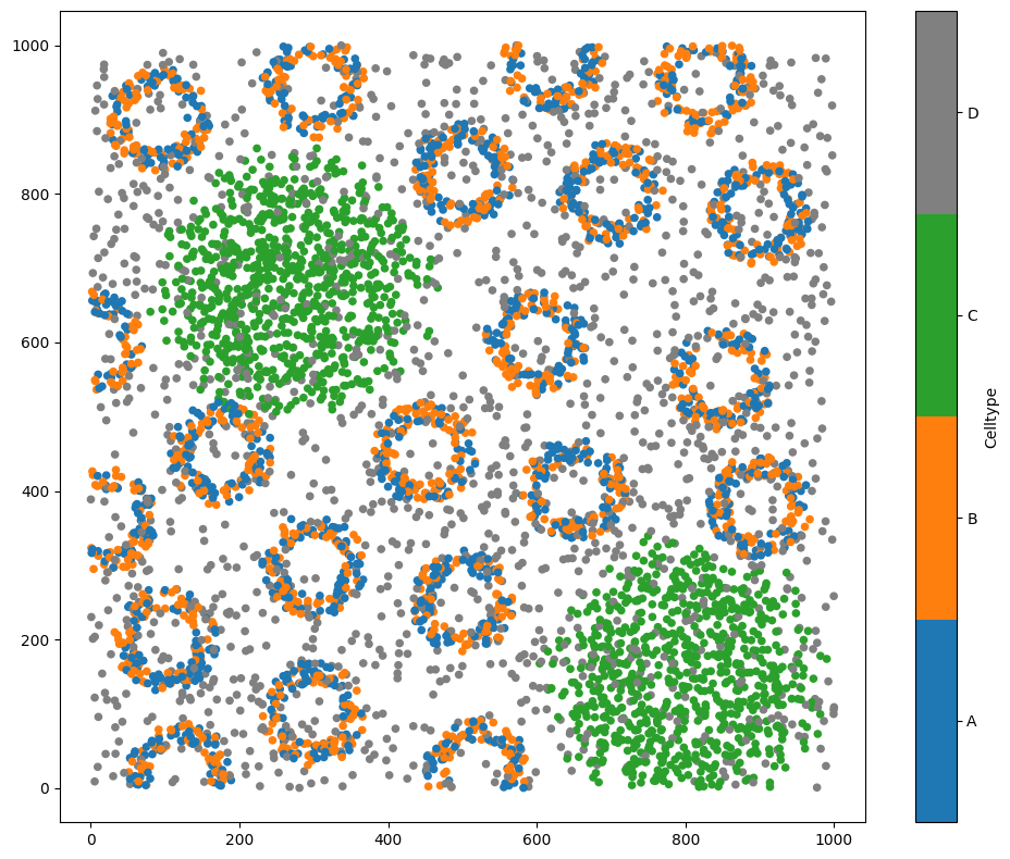
example_domain = ms.datasets.load_example_domain('Synthetic-Points-Architecture')

# Visualise the example domain with the 'Celltype' label
ms.visualise.visualise(example_domain, 'Celltype')

MuSpAn domain loaded successfully. Domain summary:
Domain name: Architecture
Number of objects: 5991
Collections: ['Cell centres']
Labels: ['Celltype']
Networks: []
Distance matrices: []

(<Figure size 1000x800 with 2 Axes>, <Axes: >)

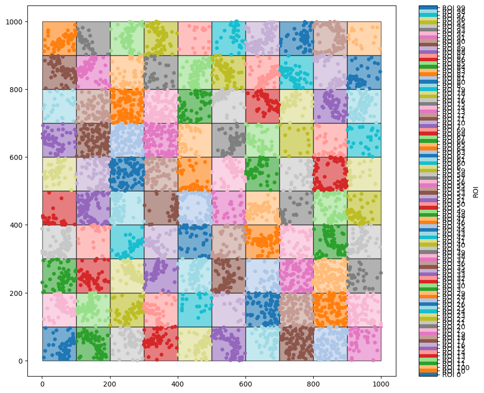
Similar to our first tutorial on tiling, we will be using the region_based submodule. Namely, we can use the generate_quadrats function in this submodule. Luckily (almost by design!) all parameters of generate_quadrats are identical to generate_hexgrid. Therefore, the previous tutorial can be used to checkout how we might want to play with boundaries and labels.

Here, we will just demonstrate using this function with side_length=100.

# Generate a quadrat grid within the example domain
# The grid will have a side length of 100 units
ms.region_based.generate_quadrats(example_domain, side_length=100, regions_collection_name='Quadrats', region_label_name='ROI')

# Visualise the generated quadrats within the example domain
ms.visualise.visualise(example_domain, 'ROI')

(<Figure size 1000x800 with 2 Axes>, <Axes: >)

# Visualise the grid within the example domain, focusing on the region counts for label 'A'
ms.visualise.visualise(example_domain, 'region counts: A', objects_to_plot=('collection', 'Quadrats'))

# Visualise the 'Celltype' label within the example domain, overlaying the cell centres
ms.visualise.visualise(example_domain, 'Celltype', objects_to_plot=('collection', 'Cell centres'), ax=plt.gca(), marker_size=10)

(<Figure size 1000x800 with 3 Axes>, <Axes: >)

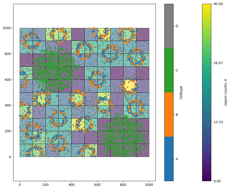
We have made square shape-like objects that have created to tile the doamin. These regions can be used for futher investigations, such as hotspot analysis or can be used to create MuSpAn subdomains using the crop_domain function in the helpers submodule.

As before we recommend checking out our documentation on generate_quadrats to get the most out of this functionality.