Cropping a domain

MuSpAn allows you to take a large domain and crop out a subset of it to form a new domain. This may be very useful when, for example, you want to restrict your focus to a specific area of your data, or if you want to see how some spatial metric varies across a large sample.

In this tutorial, we’ll explore how we can trim a large domain down into a smaller one (or many smaller ones).

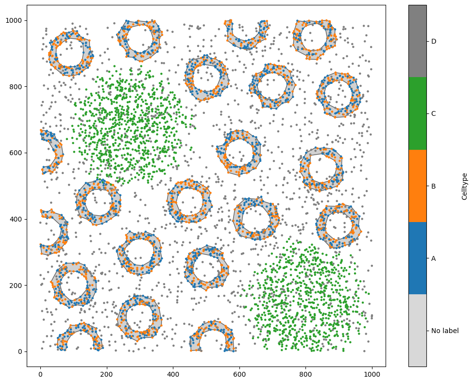
Let’s start by loading in a domain, and making sure that it has some points and some shapes in it. We’ll make the shapes using alpha shapes, so that our ‘crypts’ of A and B cells are represented with a boundary shape.

import muspan as ms
import matplotlib.pyplot as plt

# Load in a domain and make some ring shapes in it
domain = ms.datasets.load_example_domain('Synthetic-Points-Architecture')
type_A_cells = ms.query.query(domain,('label','Celltype'),'is','A')
type_B_cells = ms.query.query(domain,('label','Celltype'),'is','B')
rings = ms.query.query_container(type_A_cells,'OR',type_B_cells)
new_IDs = domain.convert_objects(rings,collection_name='New object',return_IDs=True,object_type='shape',conversion_method='alpha shape',conversion_method_kwargs=dict(alpha=20))

ms.visualise.visualise(domain,'Celltype',marker_size=5)

MuSpAn domain loaded successfully. Domain summary:
Domain name: Architecture
Number of objects: 5991
Collections: ['Cell centres']
Labels: ['Celltype']
Networks: []
Distance matrices: []

(<Figure size 1000x800 with 2 Axes>, <Axes: >)

Let’s use one of those new IDs to make a new domain containing all the points inside a specific crypt. We’ll pick out one ID (object 5991, the first of the alpha shapes that we’ve just added) and see how it looks in the whole domain.

ms.visualise.visualise(domain,objects_to_plot=[new_IDs[0]],show_boundary=True)
plt.title(f'Object ID {new_IDs[0]}')

Text(0.5, 1.0, 'Object ID 5991')

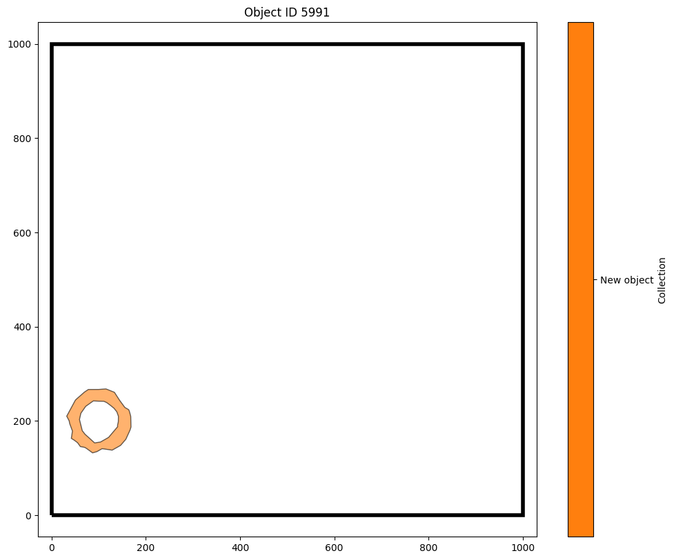
Great, we know which object ID 5991 is now. Now let’s crop the domain down to that object.

outputs = ms.helpers.crop_domain(domain, [5991])
tiny_domain = outputs[5991]
ms.visualise.visualise(tiny_domain,'Celltype',show_boundary=True)

(<Figure size 1000x800 with 2 Axes>, <Axes: >)

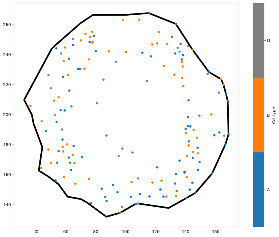
There we have it - a brand new domain whose boundary matches the outside of the shape we just passed it. Notice a couple of things here. First, the labels in tiny_domain have been inherited from the big domain - we were able to colour the points by 'Celltype' without any difficulty.

The other, potentially more misleading thing, is that crop_domain didn’t immediately return a new domain - instead, it returned a dictionary that we called outputs, and we pulled our new domain out using the key 5991. This might seem a strange syntax when you’re cropping out a single domain, but makes much more sense if we crop out many different domains at once:

outputs = ms.helpers.crop_domain(domain, new_IDs)
print(outputs)
#ms.visualise.visualise(tiny_domain,'Celltype',show_boundary=True)

{np.int64(5991): <muspan.domain.domain object at 0x1693598b0>, np.int64(5992): <muspan.domain.domain object at 0x16a347440>, np.int64(5993): <muspan.domain.domain object at 0x30e5232c0>, np.int64(5994): <muspan.domain.domain object at 0x16fdaed80>, np.int64(5995): <muspan.domain.domain object at 0x16ff13cb0>, np.int64(5996): <muspan.domain.domain object at 0x16a2c3740>, np.int64(5997): <muspan.domain.domain object at 0x30e663470>, np.int64(5998): <muspan.domain.domain object at 0x16a420bf0>, np.int64(5999): <muspan.domain.domain object at 0x16fdae900>, np.int64(6000): <muspan.domain.domain object at 0x16a421f10>, np.int64(6001): <muspan.domain.domain object at 0x16a2c0d70>, np.int64(6002): <muspan.domain.domain object at 0x16a4233b0>, np.int64(6003): <muspan.domain.domain object at 0x16a2c2ab0>, np.int64(6004): <muspan.domain.domain object at 0x16a573710>, np.int64(6005): <muspan.domain.domain object at 0x16a44c7d0>, np.int64(6006): <muspan.domain.domain object at 0x16a2c36b0>, np.int64(6007): <muspan.domain.domain object at 0x16a573fe0>, np.int64(6008): <muspan.domain.domain object at 0x16a2c1ee0>, np.int64(6009): <muspan.domain.domain object at 0x16a132f30>, np.int64(6010): <muspan.domain.domain object at 0x16fc447d0>, np.int64(6011): <muspan.domain.domain object at 0x16a44e9c0>}

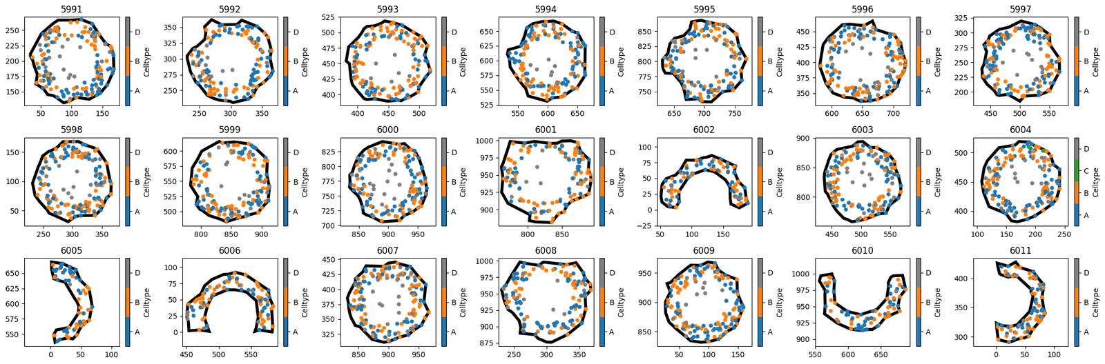
outputs now contains a dictionary of 21 domains, corresponding to the 21 IDs in the list of new_IDs. In general, we don’t have to pass specific object IDs here - any query like object that returns some shapes will result in a new domain for each shape.

fig, axes = plt.subplots(nrows=3,ncols=7,figsize=(21,7))
i, j = (0,0)
for key in outputs:
    this_domain = outputs[key]
    ms.visualise.visualise(this_domain,'Celltype',ax=axes[j,i],show_boundary=True)
    axes[j,i].set_title(key)
    i = i + 1
    if i > 6:
        i = 0
        j = j + 1

A situation where we might be interested in cropping the domain is when we’re using a lattice, for example. Let’s add a hexagonal lattice to our original domain, and use it to crop out a single hexagon.

hex_IDs = ms.region_based.generate_hexgrid(domain,150)
ms.visualise.visualise(domain,'ROI')

(<Figure size 1000x800 with 2 Axes>, <Axes: >)

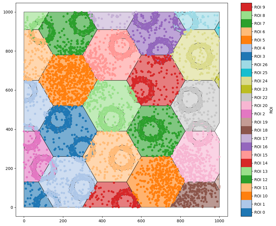
generate_hexgrid has created hexagons with the label ‘ROI’. Let’s use a query to get the hexagon with ROI 14, and crop out a new domain with that as the boundary. Before we do, note that every object in ROI 14 has also been assigned this as a label - if we just get all the objects with ROI equal to ‘ROI_14’, we’ll find a lot of objects.

ms.visualise.visualise(domain,'ROI',objects_to_plot=('ROI','ROI 14'))

(<Figure size 1000x800 with 2 Axes>, <Axes: >)

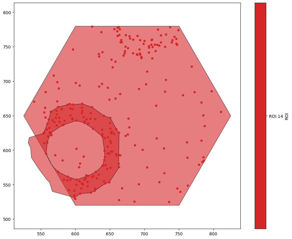
As a result, we’ll use a more complex query to get the ID of the hexagon we’re interested in.

q14 = ms.query.query(domain,'ROI','is','ROI 14')
qHex = ms.query.query(domain,('collection',),'is','Hexgrid')
our_hexagon = q14 & qHex
ms.visualise.visualise(domain,'ROI',objects_to_plot=our_hexagon,show_boundary=True)

(<Figure size 1000x800 with 2 Axes>, <Axes: >)

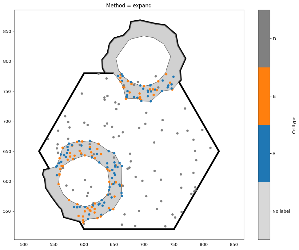
When cropping to this hexagon, we have a choice to make - the hexagon intersects with some of our crypt shapes. Do we want these shapes to be excluded from the new domain? Do we want to crop them? Do we want to expand the hexagon so that they’re kept intact? Fortunately, MuSpAn allows us to choose which option we like best.

options = ['exclude','clip','expand']

fig, axes = plt.subplots(ncols=3,figsize=(21,7))
for i, option in enumerate(options):
    new_domain_dict = ms.helpers.crop_domain(domain, our_hexagon, handle_intersecting_objects=option)
    the_key = list(new_domain_dict.keys())[0]
    ms.visualise.visualise(new_domain_dict[the_key],'Celltype',ax=axes[i],show_boundary=True)
    axes[i].set_title(f'Method = {option}')
    print(f'Method {option} - Area: {new_domain_dict[the_key].boundary.area}')
    print(f'Method {option} - Number of objects: {new_domain_dict[the_key].n_objects}')

Method exclude - Area: 58456.71475544251
Method exclude - Number of objects: 252
Method clip - Area: 58456.71475544251
Method clip - Number of objects: 254
Method expand - Area: 69430.46241487308
Method expand - Number of objects: 254

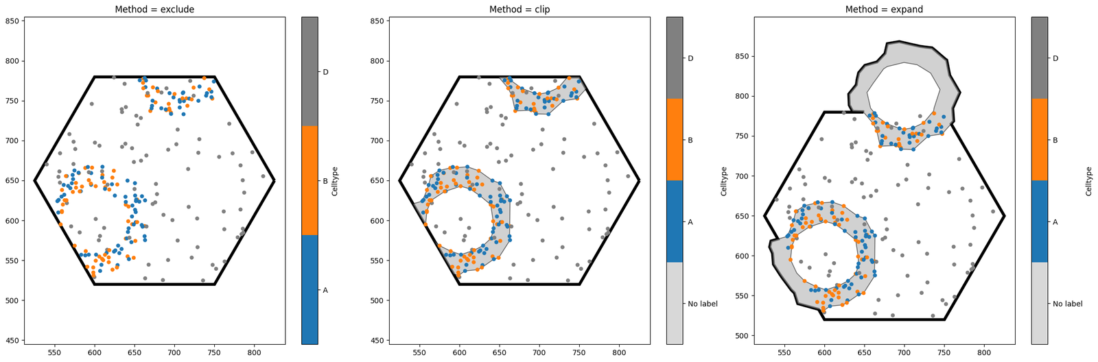
Notice the key differences between the three options. exclude is the strictest, and will completely discard any shape which intersects with the object boundary. By contrast, clip leads to a domain with the same area as exclude, but any objects intersecting with the boundary will be clipped (note that this may turn one object into many, if the clipped shape is no longer connected). Finally, expand is the most tolerant method, ensuring that all our shapes remain unaltered at the expense of increasing the domain area. The best method to choose will depend on your use case.

Finally, there is one more way of cropping to this hexagon. Notice that in the very red plot a few cells up (where we visualised all objects with the label ROI equal to ROI 14), only one of the two crypt shapes shown here was shown. This is because when we generate a hexgrid, objects are assigned a single label based on the region that their centroid is contained in. We can crop the domain to these objects immediately by specifying crop_method='label' in crop_domain.

new_domain_dict = ms.helpers.crop_domain(domain,crop_method='label',label_name='ROI')
print(new_domain_dict)

{np.str_('ROI 0'): <muspan.domain.domain object at 0x30e9ec560>, np.str_('ROI 1'): <muspan.domain.domain object at 0x16fdac8c0>, np.str_('ROI 10'): <muspan.domain.domain object at 0x30ee61970>, np.str_('ROI 11'): <muspan.domain.domain object at 0x30ef32de0>, np.str_('ROI 12'): <muspan.domain.domain object at 0x30eb78140>, np.str_('ROI 13'): <muspan.domain.domain object at 0x30ebc98e0>, np.str_('ROI 14'): <muspan.domain.domain object at 0x30e3a0980>, np.str_('ROI 15'): <muspan.domain.domain object at 0x30e325190>, np.str_('ROI 16'): <muspan.domain.domain object at 0x16a238200>, np.str_('ROI 17'): <muspan.domain.domain object at 0x30ed0b560>, np.str_('ROI 18'): <muspan.domain.domain object at 0x30ec79730>, np.str_('ROI 19'): <muspan.domain.domain object at 0x16fdadf40>, np.str_('ROI 2'): <muspan.domain.domain object at 0x30ec78140>, np.str_('ROI 20'): <muspan.domain.domain object at 0x30ebad280>, np.str_('ROI 22'): <muspan.domain.domain object at 0x30f135ac0>, np.str_('ROI 23'): <muspan.domain.domain object at 0x30ec5afc0>, np.str_('ROI 24'): <muspan.domain.domain object at 0x30e663a10>, np.str_('ROI 25'): <muspan.domain.domain object at 0x30ec5aa20>, np.str_('ROI 26'): <muspan.domain.domain object at 0x30ec40aa0>, np.str_('ROI 3'): <muspan.domain.domain object at 0x30eccd160>, np.str_('ROI 4'): <muspan.domain.domain object at 0x30ec5a810>, np.str_('ROI 5'): <muspan.domain.domain object at 0x30eb6fa40>, np.str_('ROI 6'): <muspan.domain.domain object at 0x30ec95dc0>, np.str_('ROI 7'): <muspan.domain.domain object at 0x16a4c56d0>, np.str_('ROI 8'): <muspan.domain.domain object at 0x30e341250>, np.str_('ROI 9'): <muspan.domain.domain object at 0x30e2b9490>}

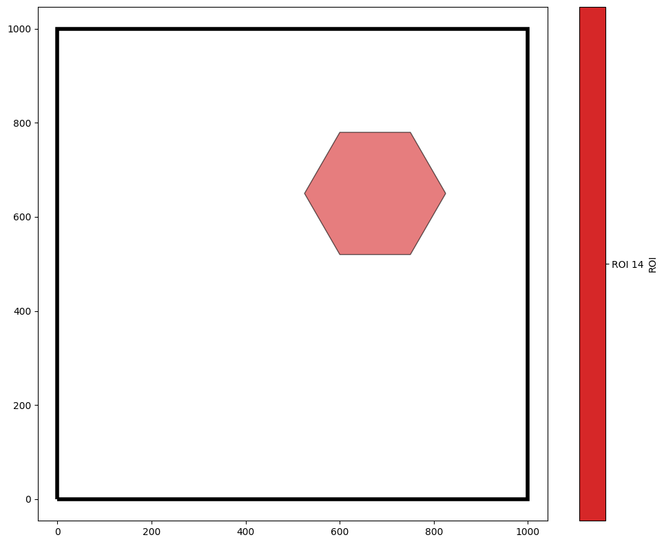
This has used the ROI label to crop a new domain based on every possible value of the label ROI. This is in general substantially faster than repeatedly iterating over shapes and cropping to them. Cropping by label will find all shapes with the same value of that label, and create a new domain which encloses all of them. The new domain boundary is the convex hull around the points/shapes contained within that label.

ms.visualise.visualise(new_domain_dict['ROI 14'],'Celltype',show_boundary=True)

(<Figure size 1000x800 with 2 Axes>, <Axes: >)

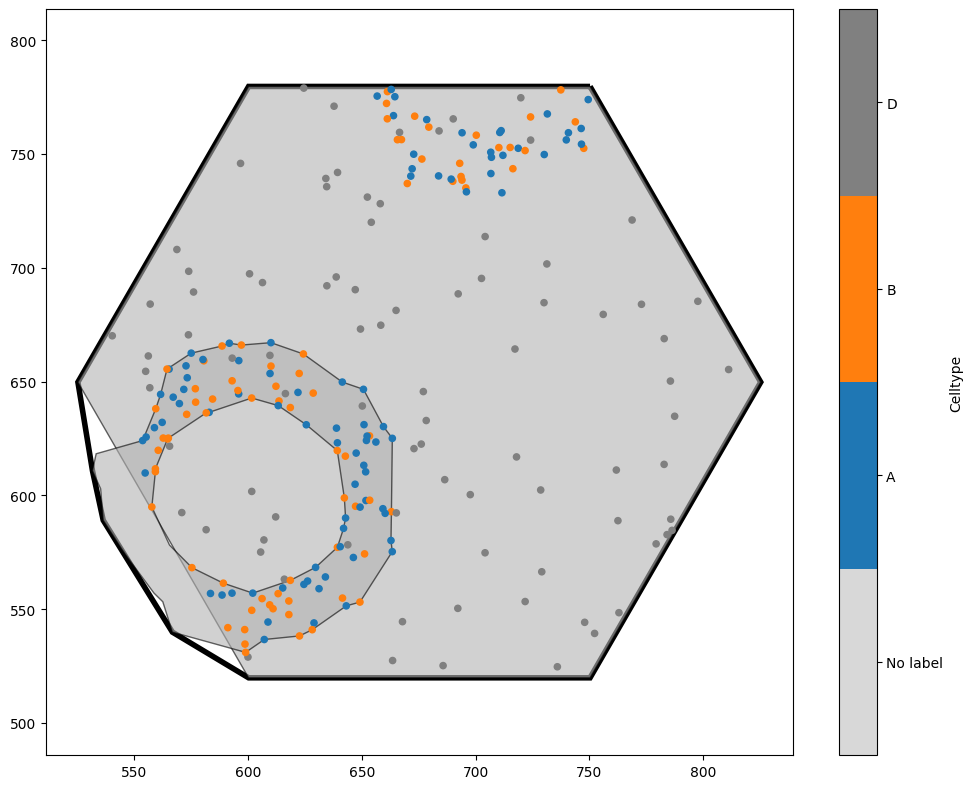
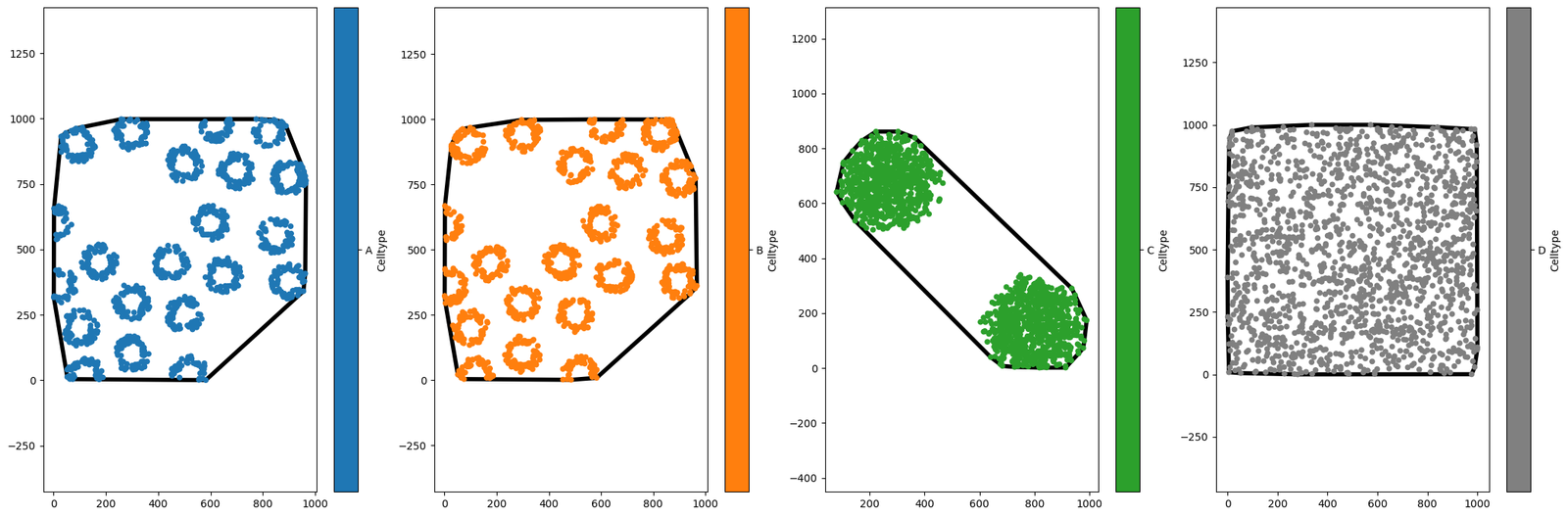
In this example, because we generated a hexgrid which added new shapes to the domain, we’ve picked up a giant hexagon within our new domain! If we wanted, we could now delete this (remember that the hexagon is in a different collection to the other objects, which would make it straightforward to remove). This cropping functionality is extremely useful in situations where we have local neighbourhoods - for instance, if we had assigned each cell centre a neighbourhood ID (see, for instance, the ‘Paper examples’ tutorial for making Figure 5 of the MuSpAn paper). It means that we can crop objects out of our domain even without having a shape that defines the boundary we wish to crop to. As an example, let’s make new domains which contains only points with the same cell type.

new_domain_dict = ms.helpers.crop_domain(domain,crop_method='label',label_name='Celltype')
print(new_domain_dict)

fig, axes = plt.subplots(ncols=4,figsize=(21,7))
for i, option in enumerate(['A','B','C','D']):
    ms.visualise.visualise(new_domain_dict[option],'Celltype',ax=axes[i],show_boundary=True)

{np.str_('A'): <muspan.domain.domain object at 0x30ec95400>, np.str_('B'): <muspan.domain.domain object at 0x30ea26ed0>, np.str_('C'): <muspan.domain.domain object at 0x1699226f0>, np.str_('D'): <muspan.domain.domain object at 0x30ea798b0>}

Just for fun, let’s see one of these plots again!

options = ['expand']
for i, option in enumerate(options):
    new_domain_dict = ms.helpers.crop_domain(domain, our_hexagon, handle_intersecting_objects=option)
    the_key = list(new_domain_dict.keys())[0]
    ms.visualise.visualise(new_domain_dict[the_key],'Celltype',show_boundary=True)
    plt.gca().set_title(f'Method = {option}')
    print(f'Method {option} - Area: {new_domain_dict[the_key].boundary.area}')
    print(f'Method {option} - Number of objects: {new_domain_dict[the_key].n_objects}')

Method expand - Area: 69430.46241487308
Method expand - Number of objects: 254